
We start over with a general second order ordinary differential equation

and this time we won’t impose any restrictions on the right-hand side. We express 


The variables 


where 


with
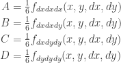
and 


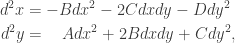
We have that

Polarisation gives that
which are geodesic equations of a connection of the two-dimensional tangent spaces in the three-dimensional projectivised tangent bundle (also called the manifold of elements). Each tangent space has coordinates 
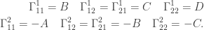
We collect the Christoffel symbols in a connection one-form

We calculate the curvature two-form 


where 
We extend the tangent spaces of the base manifold to projectives planes by adding a line at infinity in each tangent space. The points in the affine part of the projective tangent spaces have homogenous coordinates 


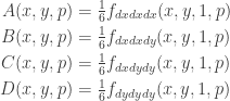
At an element 


with

The curvature of the osculating connection of
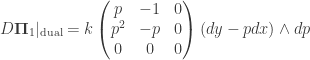
The curvature form of the primal osculating connection is characterised by that all lines through the origin are invariant. The curvature form of the dual osculating connection is characterised by that all points on the line 
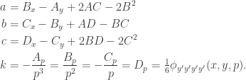
From the curvatures we get two invariants in the bundle:

which are dual to each other.
