We start over with a general second order ordinary differential equation
and this time we won’t impose any restrictions on the right-hand side. We express and which gives that
The variables and denote velocity and are tangent space coordinates. The variables and denote acceleration and are jet space (of curves) coordinates. Since the right-hand side is simultaneous homogeneous of degree 3 in and we instead consider equations of the form
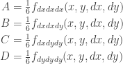
where is homogeneous of degree 3 in and , that is . Euler’s theorem then gives that we can express
with
and are homogeneous of degree 0 in and . We put and consider to be functions in and :
We have that
Polarisation gives that
which are geodesic equations of a connection of the two-dimensional tangent spaces in the three-dimensional projectivised tangent bundle (also called the manifold of elements). Each tangent space has coordinates and and the projectivised tangent bundle has coordinates and . We can read off the Christoffel symbols of this connection as
We collect the Christoffel symbols in a connection one-form
We calculate the curvature two-form by applying the exterior covariant derivative to the connection one-form
where means ordinary exterior derivative and
We extend the tangent spaces of the base manifold to projectives planes by adding a line at infinity in each tangent space. The points in the affine part of the projective tangent spaces have homogenous coordinates and points on the line at infinity have homogenous coordinates . We also extend the connection into two projective connections and :
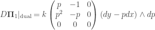
At an element a connection in the bundle defines an osculating connection in the base manifold by regarding as constant. Also an osculating connection is defined in the dual manifold by regarding as constant. The curvature of the osculating connection of in the base manifold is
with
The curvature of the osculating connection of in the dual manifold is
The curvature form of the primal osculating connection is characterised by that all lines through the origin are invariant. The curvature form of the dual osculating connection is characterised by that all points on the line are invariant. These two relations are dual and it follows that the two osculating connections are dual.
From the curvatures we get two invariants in the bundle:
We start with a general second order ordinary differential equation
and express and which gives that
The variables and denote velocity and are tangent space coordinates. The variables and denote acceleration and are jet space (of curves) coordinates. Since the right-hand side is simultaneous homogeneous of degree 3 in and we instead consider equations of the form
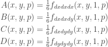
where is homogeneous of degree 3 in and , that is . Euler’s theorem then gives that we can express
with
and are homogeneous of degree 0 in and .
We now make the simplifying assumption that do not depend on and and hence are functions in and only. (This means that we are restricting to equations with right-hand side that is a third degree polynomial in the first derivative, .)
We have that
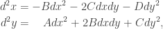
Polarisation gives that
which are geodesic equations and we can read off the Christoffel symbols as
We collect the Christoffel symbols in a connection one-form
We calculate the curvature two-form by applying the exterior covariant derivative to the connection one-form
where means ordinary exterior derivative and
We read off the Riemann tensor components
By contracting the Riemann tensor we get the components of the Ricci quadratic form
The Ricci quadratic form is the two-dimensional analogue of the Schwarzian derivative and allows us to construct a projective structure for each geodesic. Set
and let
The vector will trace out a curve in . Since the acceleration is parallel to the curve will be planar. The containing plane defines homogeneous coordinates on the geodesic and this gives the geodesic a projective structure.
Since the Ricci quadratic form defines a projective structure on every solution curve we might wonder if these projective structures fit together to also give a two-dimensional projective structure on the -plane. To investigate this we reinterpret the Ricci form as a one-form valued one-form and express it as a row vector of one-forms
We apply the exterior covariant derivative to this form
with
is a one-form valued two-form, which perhaps can be called the Bianchi form, and is the obstruction of the integrability of the one-dimensional projective structures into a two-dimensional projective structure. This can, perhaps, be understood geometrically in the following way. Parallel transport a plane around a loop in . After the parallel transport the plane might have become tilted compared to its initial position. The form which when evaluated on a bivector at a point gives a covector. The null direction of this covector is a rotation axis and the magnitude of the covector is the rotational velocity around this axis in .
When vanishes, a plane when parallel transported in a tangential direction in will always be the tangent plane of an integral surface. The Ricci quadratic form is the centroaffine fundamental form of this surface. The solution curves will be curves on the surface cut by planes through the origin and will be homogeneous coordinates thus giving a projective structure to the -plane.
If the surface is projected from the origin onto a plane not passing through the origin, the solution curves are projected onto straight lines. This gives a diffeomorphism that maps the differential equation to the trivial one.
where is the covariant exterior derivative and means the ordinary exterior derivative.
The Ricci quadratic form is
which is the centroaffine fundamental form of a centered elliptical cylinder in . The coordinates and parameterise the cylinder, is the angular coordinate and is the longitudinal coordinate on the cylinder. The solution curves are curves that are given by intersecting the cylinder with planes through the origin.
In this way becomes homogenous coordinates on the -plane and realises the projective structure inherent in the differential equation. The differential equation thus has the symmetry group .
We can extend the connection to a connection in . We define cylindrical coordinates , where is the angular coordinate, is the longitudinal coordinate and is the radial coordinate. In these coordinates we define the connection one-form as
where the upper left -submatrix is , the rightmost column is the standard column one-form and the bottom row is the Ricci quadratic form expressed as a row one-form. A geodesic of this connection that starts parallel to a coordinate cylinder () will stay on the cylinder and has its acceleration vector parallel to the position vector and so will trace out an ellipse that is the intersection of the cylinder and a plane through the origin.
The curvature of this connection vanishes:
confirming that the connection defines a projective structure on the -plane.
We will investigate the motion of point vortices and dipole vortices on a Riemann surface. We’ll start with the point vortex case and will mainly follow the well-written exposition given by Björn Gustafsson in Vortex motion and geometric function theory: the role of connections.
The setup is that we have a Riemann surface of genus and equipped with a conformal metric . On this surface we specify point vortices located at points with strengths given by real numbers such that and a steady background flow defined by periods and .
We construct a Green function for the Riemann surface which is a solution to
,
where is the Laplace operator, is a point source at and is a constant function acting as a background sink.
The Green function can be expanded as
The stream function is constructed by adding together the individual Green functions
where is the harmonic conjugate of the background flow defined by the given periods and . The complex potential consists of the velocity potential and the stream function related by .
The complex potential can be expanded at as
and we have that
We note that the expansion is dependent on the coordinate system. This means that is not a proper one-form but rather an affine connection. If is a holomorphic coordinate change then transforms as , where is the affine derivative of .
The differential of is then expanded as
The complex flow vector field is given by using the metric to convert the conjugate of the differential component of to the component of the vector field
It is reasonable to expect a vortex to flow along the fluid, but since the velocity field is singular at we investigate this further by expanding the conjugated derivative of at
We might to try to renormalise this expression by simply discarding the complex pole term and then letting , keeping only the finite part to be the velocity of the vortex point
But since is not a proper one-form this won’t do, the calculation will be dependent on the coordinate system. We remedy this by noting that there is a special coordinate system: the normal coordinate system in which . We thus choose the renormalisation to be the in the normal coordinate system, treat this as the component of a one-form and translate it to our original coordinate system. We then get
This can be written as
where and . These are both affine connection component functions and since the difference between two affine connections is a proper one-form we see that our renormalised expression for the vortex motion is well-defined.
We now continue to investigate the motion of dipole vortices on the Riemann surface .
On the surface we specify dipole vortices located at points with strengths and orientations given by complex numbers . We also specify a steady background flow defined by periods and .
The absolute strength of a dipole vortex at is and the orientation is . If is a holomorphic coordinate change then the strength-and-orientation numbers transform according to .
We let mean the exterior derivative with respect to . The -differential of a Green function is then a stream function on the Riemann surface depending on and where is a complex variable denoting the strength-and-orientation of the stream field.
We have that
where is the conjugate value of . This means that can be understood as a “Green function” of a dipole. We also see that is harmonic for . The decomposition of
is then the decomposition of into a meromorphic function and an antimeromorphic function . This means that is the complex potential of the flow.
The dipole complex potential has a pole at and is expanded as
The complex potential of the total flow is constructed from the differentiated Green function and the periods by
where is the potential of the background flow defined by the given periods and . At the complex potential can be expanded as
where
The differential of is then expanded as
The expansion is dependent on the coordinate system. So the form is not a proper differential quadratic form but rather a projective connection. If is a holomorphic coordinate change then transforms as , where is the Schwarzian derivative of .
The velocity field component at is then
where is the conjugate value of . We renormalise the velocity at by choosing the expansion to be in the normal coordinate system, discarding the pole, treating to be the component of a differential quadratic form and then translating it to the original coordinate system. We get
which can be written as
where and . These are both projective connection component functions and since the difference between two projective connections is a differential quadratic form we see that the dipole vortex motion is indeed well-defined.
It is reasonable to expect the strength-and-orientation numbers to be affected by the flow. The is equivalent to the component of a tangent vector and so its time evolution should be governed by the acceleration vector at the point, . To investigate this further we specialise to the case where there is only one dipole vortex at with strength-and-orientation number and no background flow. The complex potential is then
and the motion of the dipole is given by
where
By setting and substituting we get the equation
where and . Solving for gives
If we instead substitute we can rewrite this as
This is a geodesic equation with Christoffel symbols
We conclude that the dipole moves on a geodesic of a connection generated by the Green function.
Let be a vector field on the Euclidean line . Expressed in a coordinate the vector field is . The logarithm of the component value at each point of the vector field is the fundamental Euclidean invariant
We now let denote the component of the vector field, and so . Let be a diffeomorphism of the Euclidean line. The vector field is then pushed-forward by . By taking the difference between the fundamental invariants of the pushed-forward vector field and the original vector field,
we recover the logarithm of the derivative as the fundamental Euclidean invariant of a diffeomorphism.
From the invariant further invariants can be constructed by differentiating with respect to the vectorfield
Let be another vector field. Then we have that
which shows that is a cocycle on .
The invariant is also an invariant for vector fields on the affine line . For a diffeomorphism of the affine line we get an invariant one-form by taking the difference of the invariants of the pushed-forward and original vector fields:
By differentiating with respect to the vector field we get another affine invariant
This is also a cocycle but instead of showing this by direct calculation, we assume that the diffeomorphism is generated by the flow the of the vector field
where is a fixed parameter of the flow. Then
which shows that is the first order term of and since is a diffeomorphism group cocycle, it follows that is its corresponding vector field algebra cocycle.
We now consider a vector field on the projective line and lift it to homogeneous coordinates by
This gives a constant area-velocity vector field which means that the acceleration vector field is a central field. The ratio between the acceleration vector and the position vector then gives the fundamental projective invariant of this vector field:
Again, by pushing forward the vector field by a diffeomorphism and taking the difference of the invariants we get an invariant of the diffeomorphism, the Schwarzian derivative:
Differentiating gives another projective invariant of the vector field
And this invariant then has the interpretation that it gives the intrinsic change of the acceleration/position ratio of the lifted vector field.
Since is related to the cocycle in the same way as the cocycle is related to the cocycle (and also to ) it follows that is a cocycle. It is the vector field algebra cocycle counterpart of the Schwarzian diffeomorphism group cocycle, the Gelfand-Fuchs cocycle.
For a diffeomorphism between two Euclidean lines, the derivative is an invariant in the sense that to calculate the derivative we fix Euclidean coordinate systems on the domain and on the range and the calculated value will not depend on the choice of coordinate systems.
For a diffeomorphism between affine lines, things are not that simple, the calculated value of the derivative will be dependent on the affine coordinate systems it is computed in. To find an invariant expression we look at the fundamental invariant of the affine line, the three-point ratio:
We put and . Then and the ratio of the images of the three points is then
and so the one-form is an invariant that measures how much the diffeomorphism deviates from being an affine transformation.
Now let be a coordinate on the range and thus . We can express the derivatives of as
and the invariant one-form can be reexpressed as . Each of the two quotients is invariant under affine coordinate changes so in fact any function would define an invariant of the diffeomorphism, but it is only by taking the difference that the second order differentials cancel and we get an invariant that is a one-form on the tangent space.
Let’s carry out this calculation, which is in a sense the last calculation carried out backwards. Since the second differential of is , we get
as expected.
Moving on to instead study a diffeomorphism between projective lines, we now want to see how the cross ratio
changes under the diffeomorphism. We put , , and calculate that . On the range space we want to make use of the availability of homogenous coordinates and define a lift of to a vector by
This lift has the property that the curve has constant angular momentum and thus the acceleration vector is parallel to the position vector . The cross ratio can be calculated in homogenous coordinates as
We have that
The cross products become
and the cross ratio of the image points is
So we get a quadratic form, the Schwarzian derivative, that tells us how much the diffeomorphism deviates from being a projective transformation. The coefficient is calculated as
and the Schwarzian derivative when directly expressed in derivatives of becomes
We have already given above the first and second derivative of expressed as differentials of and . The third derivative then can also be reexpressed as
and the Schwarzian derivative then becomes
Thus we see, just as in the affine case, that the invariant form for the diffeomorphism is a difference between two separately invariant higher order forms, one on the range and one on the domain.
We now define and . For a composition of diffeomorphisms , we get
and we have shown the cocycle condition for the Schwarzian derivative.
We start with a Lie group . An element acts on an external vector by . Let be generated by a vector at the identity , . By differentiating, with , the velocity of is
This can also be interpreted that is the parallel transport of to . The velocity of can then be expressed as
so we see that the action of an element of the Lie algebra on a vector generates a velocity of this vector.
Now let be differentiation in some independent direction and let be a corresponding vector in the Lie algebra. The -derivative of is then multiplication with :
Swapping the order of differentiation gives
and combining these gives
The operator is the exterior (covariant) derivative squared and computes the torsion of the action (i.e. the connection) of the Lie group. The righthand side is of course the usual commutator in the Lie algebra. We can thus reexpress the last expression as
The purpose of this post is to show how the cross ratio can be understood as a generalisation of the corresponding invariants in Euclidean and affine geometry and how it is closely related to the concept of a point frame. For the Euclidean line , a point frame is a single point and it allows us to specify a Euclidean invariant of another point with respect to :
So if we consider and to be coordinates in a Euclidean coordinate system, then is simply the coordinate of in the coordinate system with as its origin. This is invariant under non-reflection Euclidean coordinate changes.
Moving on to the affine line , we want to make a corresponding construction that is invariant under affine coordinate changes. Thus we extend the point frame into an affine point frame which consists of two points and define an invariant of a point with respect to this frame to be
This can be interpreted to be the coordinate of in the coordinate system with as its origin and as its unit point.
For the projective line we add a third point which makes the frame into a projective frame . The point is to be understood as the point at infinity and allows us to define an affine coordinate system with as its origin and as its unit point. The coordinate of some point in this coordinate system is
Thus the cross ratio of four points is the coordinate value of one of the points with respect to the projective frame defined by the other three points. The projective frame gives the additional structure missing in the projective geometry needed to be able to compute an invariant coordinate value and specialises the projective line into an Euclidean line.
A projective frame with three points which we now denote by uniquely determines an element of . This matrix is constructed by choosing homogenous coordinates of the three points rescaled such that
Then the corresponding element in is
Whether we interpret the third point in a projective frame as a point at infinity or as a midpoint of the other two points depends on the circumstance and is a matter of what is most convenient. The two interpretations are equivalent since the midpoint and the infinity point are harmonic conjugates with respect to the two other points of the frame. If we want to emphasis the equivalence of the midpoint and the infinity point we can include both in the frame and thus define a projective frame to be four points with a harmonic cross ratio.


 and
and  which gives that
 and
and  denote velocity and are tangent space coordinates. The variables
  and
and  denote acceleration and are jet space (of curves) coordinates. Since the right-hand side is simultaneous homogeneous of degree 3 in
 is homogeneous of degree 3 in
  . Euler’s theorem then gives that we can express
 are homogeneous of degree 0 in
  and consider
  and
and  :
:

 and
and 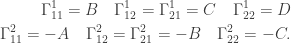

 by applying the exterior covariant derivative
  to the connection one-form
 means ordinary exterior derivative and
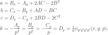
 and points on the line at infinity have homogenous coordinates
  . We also extend the connection into two projective connections
  and
and  :
:

 a connection in the bundle defines an osculating connection in the base manifold by regarding
  as constant. Also an osculating connection is defined in the dual manifold by regarding
  as constant. The curvature of the osculating connection of

 are invariant. These two relations are dual and it follows that the two osculating connections are dual.
 and
and  only. (This means that we are restricting to equations with right-hand side that is a third degree polynomial in the first derivative,
  .)
.)


 will trace out a curve in
  . Since the acceleration
  is parallel to

 is a one-form valued two-form, which perhaps can be called the Bianchi form, and is the obstruction of the integrability of the one-dimensional projective structures into a two-dimensional projective structure. This can, perhaps, be understood geometrically in the following way. Parallel transport a plane around a loop in
  we rewrite


 .
. , where
  is the radial coordinate. In these coordinates we define the connection one-form as
 -submatrix is
  , the rightmost column is the standard column one-form and the bottom row is the Ricci quadratic form expressed as a row one-form. A geodesic of this connection that starts parallel to a coordinate cylinder (
 ) will stay on the cylinder and has its acceleration vector parallel to the position vector and so will trace out an ellipse that is the intersection of the cylinder and a plane through the origin.


 of genus
  and equipped with a conformal metric
  . On this surface we specify
  point vortices located at points
  with strengths given by real numbers
  such that
  and a steady background flow defined by
  periods
  and
and  .
. for the Riemann surface which is a solution to
 ,
, is the Laplace operator,
  is a point source at
  and
and  is a constant function acting as a background sink.


 is the harmonic conjugate of the background flow defined by the given periods
  consists of the velocity potential
  and the stream function
  related by
  .
.  as
as


 is not a proper one-form but rather an affine connection. If
  is a holomorphic coordinate change then
  , where
  is the affine derivative of
  is then expanded as


 , keeping only the finite part to be the velocity of the vortex point
 is not a proper one-form this won’t do, the calculation will be dependent on the coordinate system. We remedy this by noting that there is a special coordinate system: the normal coordinate system in which
  . We thus choose the renormalisation to be the
  in the normal coordinate system, treat this as the component of a one-form and translate it to our original coordinate system. We then get

 and
and  . These are both affine connection component functions and since the difference between two affine connections is a proper one-form we see that our renormalised expression for the vortex motion is well-defined.
 . We also specify a steady background flow defined by
  is
is  and the orientation is
  . If
. If  .
. mean the exterior derivative with respect to
  . The
. The  is then a stream function on the Riemann surface depending on
  where
where 
 is the conjugate value of
  can be understood as a “Green function” of a dipole. We also see that
  . The decomposition of
 and an antimeromorphic function
  . This means that
  is the complex potential of the flow.
 of the total flow is constructed from the differentiated Green function and the periods by
 is the potential of the background flow defined by the given periods


 is not a proper differential quadratic form but rather a projective connection. If
  , where
  is the
  is then
 is the conjugate value of
  . We renormalise the velocity at
  to be the component of a differential quadratic form and then translating it to the original coordinate system. We get

 and
and  . These are both projective connection component functions and since the difference between two projective connections is a differential quadratic form we see that the dipole vortex motion is indeed well-defined.
 . To investigate this further we specialise to the case where there is only one dipole vortex at


 and substituting
  we get the equation


 and
and  . Solving for
  gives
gives

 we can rewrite this as


 be a vector field on the Euclidean line
  . Expressed in a coordinate
  . The logarithm of the component value at each point of the vector field is the fundamental Euclidean invariant
 and so
  . Let
. Let  be a diffeomorphism of the Euclidean line. The vector field is then pushed-forward by
  . By taking the difference between the fundamental invariants of the pushed-forward vector field and the original vector field,
 further invariants can be constructed by differentiating with respect to the vectorfield
 be another vector field. Then we have that
![\displaystyle\begin{aligned} i_1([d,\partial ]) &= i_1(d\partial-\partial d)=\frac{(d\partial-\partial d)}{(d\partial-\partial d)x}(d\partial-\partial d)x=\\ &=\frac{d}{dx}d\partial x-\frac{\partial}{\partial x}\partial dx =\\ &= \frac{d}{dx}dx\frac{\partial}{\partial x}\partial x-\frac{\partial}{\partial x}\partial x\frac{d}{dx} dx =\\ &=d\frac{\partial^2x}{\partial x}-\partial\frac{d^2x}{dx}=\\ &=d\, i_1( \partial)-\partial\, i_1(d),\end{aligned}](https://s0.wp.com/latex.php?latex=%5Cdisplaystyle%5Cbegin%7Baligned%7D+i_1%28%5Bd%2C%5Cpartial+%5D%29+%26%3D+i_1%28d%5Cpartial-%5Cpartial+d%29%3D%5Cfrac%7B%28d%5Cpartial-%5Cpartial+d%29%7D%7B%28d%5Cpartial-%5Cpartial+d%29x%7D%28d%5Cpartial-%5Cpartial+d%29x%3D%5C%5C+%26%3D%5Cfrac%7Bd%7D%7Bdx%7Dd%5Cpartial+x-%5Cfrac%7B%5Cpartial%7D%7B%5Cpartial+x%7D%5Cpartial+dx+%3D%5C%5C+%26%3D%C2%A0%5Cfrac%7Bd%7D%7Bdx%7Ddx%5Cfrac%7B%5Cpartial%7D%7B%5Cpartial+x%7D%5Cpartial+x-%5Cfrac%7B%5Cpartial%7D%7B%5Cpartial+x%7D%5Cpartial+x%5Cfrac%7Bd%7D%7Bdx%7D+dx+%3D%5C%5C+%26%3Dd%5Cfrac%7B%5Cpartial%5E2x%7D%7B%5Cpartial+x%7D-%5Cpartial%5Cfrac%7Bd%5E2x%7D%7Bdx%7D%3D%5C%5C+%26%3Dd%5C%2C+i_1%28+%5Cpartial%29-%5Cpartial%5C%2C+i_1%28d%29%2C%5Cend%7Baligned%7D&bg=ffffff&fg=333333&s=0&c=20201002)
 is a cocycle on
  .
. . For a diffeomorphism


 is a fixed parameter of the flow. Then
 is the first order term of
  and since
  on the projective line
  and lift it to homogeneous coordinates
  by
by


 gives another projective invariant of the vector field
 is related to the cocycle
  in the same way as the cocycle
  ) it follows that
  between two Euclidean lines, the derivative
  is an invariant in the sense that to calculate the derivative we fix Euclidean coordinate systems on the domain and on the range and the calculated value will not depend on the choice of coordinate systems.
 between affine lines, things are not that simple, the calculated value of the derivative
  will be dependent on the affine coordinate systems it is computed in. To find an invariant expression we look at the fundamental invariant of the affine line, the three-point ratio:
![\displaystyle [x,x_1,x_\alpha]=\frac{x_\alpha-x}{x_1-x}](https://s0.wp.com/latex.php?latex=%5Cdisplaystyle+%5Bx%2Cx_1%2Cx_%5Calpha%5D%3D%5Cfrac%7Bx_%5Calpha-x%7D%7Bx_1-x%7D&bg=ffffff&fg=333333&s=0&c=20201002)
 and
and  . Then
 ![[x,x_1,x_\alpha]=\alpha](https://s0.wp.com/latex.php?latex=%5Bx%2Cx_1%2Cx_%5Calpha%5D%3D%5Calpha&bg=ffffff&fg=333333&s=0&c=20201002) and the ratio of the images of the three points is then
and the ratio of the images of the three points is then![\displaystyle \begin{aligned}[] [f(x),&f(x_1),f(x_\alpha)] =\frac{f(x+\alpha dx)-f(x)}{f(x+dx)-f(x)}\\ &=\frac{\alpha f'(x)dx+(\alpha^2/2)f''(x)dx^2+O(dx^3)}{f'(x)dx+(1/2)f''(x)dx^2+O(dx^3)}\\ &= \alpha+\frac{((\alpha^2-\alpha)/2)f''dx^2+O(dx^3)}{f'dx+O(dx^2)}\\ &= \alpha+\frac{\alpha^2-\alpha}{2}\frac{f''}{f'}dx+O(dx^2)\end{aligned}](https://s0.wp.com/latex.php?latex=%5Cdisplaystyle+%5Cbegin%7Baligned%7D%5B%5D+%5Bf%28x%29%2C%26f%28x_1%29%2Cf%28x_%5Calpha%29%5D+%3D%5Cfrac%7Bf%28x%2B%5Calpha+dx%29-f%28x%29%7D%7Bf%28x%2Bdx%29-f%28x%29%7D%5C%5C+%26%3D%5Cfrac%7B%5Calpha+f%27%28x%29dx%2B%28%5Calpha%5E2%2F2%29f%27%27%28x%29dx%5E2%2BO%28dx%5E3%29%7D%7Bf%27%28x%29dx%2B%281%2F2%29f%27%27%28x%29dx%5E2%2BO%28dx%5E3%29%7D%5C%5C+%26%3D+%5Calpha%2B%5Cfrac%7B%28%28%5Calpha%5E2-%5Calpha%29%2F2%29f%27%27dx%5E2%2BO%28dx%5E3%29%7D%7Bf%27dx%2BO%28dx%5E2%29%7D%5C%5C+%26%3D+%5Calpha%2B%5Cfrac%7B%5Calpha%5E2-%5Calpha%7D%7B2%7D%5Cfrac%7Bf%27%27%7D%7Bf%27%7Ddx%2BO%28dx%5E2%29%5Cend%7Baligned%7D&bg=ffffff&fg=333333&s=0&c=20201002)
 is an invariant that measures how much the diffeomorphism deviates from being an affine transformation.
 . Each of the two quotients is invariant under affine coordinate changes so in fact any function
  would define an invariant of the diffeomorphism, but it is only by taking the difference that the second order differentials cancel and we get an invariant that is a one-form on the tangent space.
 , we get
 between projective lines, we now want to see how the cross ratio
![\displaystyle [x,x_1,x_a,x_{a^2}]=\left.\frac{x_a-x}{x_1-x}\middle/\frac{x_a-x_{a^2}}{x_1-x_{a^2}}\right.](https://s0.wp.com/latex.php?latex=%5Cdisplaystyle+%5Bx%2Cx_1%2Cx_a%2Cx_%7Ba%5E2%7D%5D%3D%5Cleft.%5Cfrac%7Bx_a-x%7D%7Bx_1-x%7D%5Cmiddle%2F%5Cfrac%7Bx_a-x_%7Ba%5E2%7D%7D%7Bx_1-x_%7Ba%5E2%7D%7D%5Cright.&bg=ffffff&fg=333333&s=0&c=20201002)
 ,
,  and calculate that
 ![[x,x_1,x_a,x_{a^2}]=1+a](https://s0.wp.com/latex.php?latex=%5Bx%2Cx_1%2Cx_a%2Cx_%7Ba%5E2%7D%5D%3D1%2Ba&bg=ffffff&fg=333333&s=0&c=20201002) . On the range space we want to make use of the availability of homogenous coordinates and define a lift of
. On the range space we want to make use of the availability of homogenous coordinates and define a lift of  by
by

 and thus the acceleration vector is parallel to the position vector
  . The cross ratio can be calculated in homogenous coordinates as
![\displaystyle [\mathbf{v},\mathbf{v}_1,\mathbf{v}_a,\mathbf{v}_{a^2}]=\frac{(\mathbf{v}_a\times\mathbf{v})(\mathbf{v}_1\times\mathbf{v}_{a^2})}{(\mathbf{v}_1\times\mathbf{v})(\mathbf{v}_a\times\mathbf{v}_{a^2})}.](https://s0.wp.com/latex.php?latex=%5Cdisplaystyle+%5B%5Cmathbf%7Bv%7D%2C%5Cmathbf%7Bv%7D_1%2C%5Cmathbf%7Bv%7D_a%2C%5Cmathbf%7Bv%7D_%7Ba%5E2%7D%5D%3D%5Cfrac%7B%28%5Cmathbf%7Bv%7D_a%5Ctimes%5Cmathbf%7Bv%7D%29%28%5Cmathbf%7Bv%7D_1%5Ctimes%5Cmathbf%7Bv%7D_%7Ba%5E2%7D%29%7D%7B%28%5Cmathbf%7Bv%7D_1%5Ctimes%5Cmathbf%7Bv%7D%29%28%5Cmathbf%7Bv%7D_a%5Ctimes%5Cmathbf%7Bv%7D_%7Ba%5E2%7D%29%7D.&bg=ffffff&fg=333333&s=0&c=20201002)


![\displaystyle \begin{aligned}[][\mathbf{v},\mathbf{v}_1,\mathbf{v}_a,\mathbf{v}_{a^2}]&=\frac{1-a^2+\left(\frac{1}{6}-\frac{a^2}{3}+\frac{a^4}{3}-\frac{a^5}{6} \right) \lambda dx^2+O(dx^3)}{1-a+\left(\frac{1}{6}-\frac{a}{6}+\frac{a^2}{6}-\frac{a^3}{2}+\frac{a^4}{2}-\frac{a^5}{6}\right) \lambda dx^2+O(dx^3)}\\&=1+a+\left( -\frac{a^2}{3}+\frac{3a^4-2a^5}{6-6a} \right) \lambda dx^2+O(dx^3)\end{aligned}.](https://s0.wp.com/latex.php?latex=%5Cdisplaystyle+%5Cbegin%7Baligned%7D%5B%5D%5B%5Cmathbf%7Bv%7D%2C%5Cmathbf%7Bv%7D_1%2C%5Cmathbf%7Bv%7D_a%2C%5Cmathbf%7Bv%7D_%7Ba%5E2%7D%5D%26%3D%5Cfrac%7B1-a%5E2%2B%5Cleft%28%5Cfrac%7B1%7D%7B6%7D-%5Cfrac%7Ba%5E2%7D%7B3%7D%2B%5Cfrac%7Ba%5E4%7D%7B3%7D-%5Cfrac%7Ba%5E5%7D%7B6%7D+%5Cright%29+%5Clambda+dx%5E2%2BO%28dx%5E3%29%7D%7B1-a%2B%5Cleft%28%5Cfrac%7B1%7D%7B6%7D-%5Cfrac%7Ba%7D%7B6%7D%2B%5Cfrac%7Ba%5E2%7D%7B6%7D-%5Cfrac%7Ba%5E3%7D%7B2%7D%2B%5Cfrac%7Ba%5E4%7D%7B2%7D-%5Cfrac%7Ba%5E5%7D%7B6%7D%5Cright%29+%5Clambda+dx%5E2%2BO%28dx%5E3%29%7D%5C%5C%26%3D1%2Ba%2B%5Cleft%28+-%5Cfrac%7Ba%5E2%7D%7B3%7D%2B%5Cfrac%7B3a%5E4-2a%5E5%7D%7B6-6a%7D+%5Cright%29+%5Clambda+dx%5E2%2BO%28dx%5E3%29%5Cend%7Baligned%7D.&bg=ffffff&fg=333333&s=0&c=20201002)
 that tells us how much the diffeomorphism deviates from being a projective transformation. The coefficient


 and
and  . For a composition of diffeomorphisms
  , we get
 . An element
  acts on an external vector
  by
by  . Let
. Let  at the identity
  ,
,  . By differentiating, with
  , the velocity of
 is the parallel transport of
 be differentiation in some independent direction and let
  be a corresponding vector in the Lie algebra. The


 is the exterior (covariant) derivative squared
  and computes the torsion of the action (i.e. the connection) of the Lie group. The righthand side is of course the usual commutator in the Lie algebra. We can thus reexpress the last expression as
![D^2e=[de,\partial e].](https://s0.wp.com/latex.php?latex=D%5E2e%3D%5Bde%2C%5Cpartial+e%5D.&bg=ffffff&fg=333333&s=0&c=20201002)

 is simply the coordinate of
  and define an invariant of a point
 as its unit point.
 which makes the frame into a projective frame
  . The point
 uniquely determines an element of
  . This matrix is constructed by choosing homogenous coordinates of the three points
  rescaled such that

